A Qubit Is Not 0 or 1. It Is a Linear Combination of Both.

Every introduction to quantum computing makes the same mistake.

"A qubit can be 0 and 1 at the same time." The sentence is everywhere. It is short, it moves fast, and it gives you just enough intuition to feel like you understand something. But it encodes a fundamentally wrong picture of what superposition is, and that wrong picture compounds into bigger misunderstandings every step after it.

A qubit in superposition is not "both 0 and 1." It is a single mathematical object in a state that cannot be reduced to either. That distinction sounds subtle. It is not.

Here is what is actually happening, in five steps.

1. The State Has No Value. It Has a Vector.

A classical bit is binary and definite. At every moment, it is 0 or 1. A transistor conducts current or it does not. The bit always has a value.

A qubit in superposition has no value. What it has is a state:

|ψ⟩ = α|0⟩ + β|1⟩

Where α and β are complex numbers called probability amplitudes, constrained by the normalization condition:

|α|² + |β|² = 1

This is not describing two simultaneous values. It is describing one vector in a two-dimensional complex Hilbert space. The |ψ⟩ is its own mathematical entity, distinct from both |0⟩ and |1⟩.

Three things follow immediately from this:

Superposition does not mean the qubit "is both." |ψ⟩ is not a blend of |0⟩ and |1⟩ in the way gray is a blend of black and white. It is a different kind of object entirely.
α and β are complex numbers, not percentages. Their squared moduli give measurement probabilities, but the amplitudes themselves carry phase information that determines interference, and interference is where the computation lives.
When you measure, the state collapses. You get |0⟩ with probability |α|², or |1⟩ with probability |β|². Before that moment, neither outcome existed.

2. The Bloch Sphere: Every Point Is a Possible Quantum State

There is a clean geometric way to visualize all possible pure states of a single qubit. It is called the Bloch sphere.

Any pure qubit state can be written using two real parameters, θ and φ:

|ψ⟩ = cos(θ/2)|0⟩ + e^iφ·sin(θ/2)|1⟩

These two angles map to a unique point on the surface of a unit sphere:

North pole (θ = 0): the state |0⟩. Measuring gives 0 with 100% certainty.
South pole (θ = π): the state |1⟩. Measuring gives 1 with 100% certainty.
Equator (θ = π/2): maximum superposition, 50% probability for each outcome.

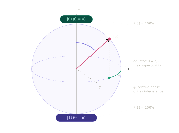
But the Bloch sphere shows something the probability numbers alone do not. The angle φ is the relative phase. It does not change measurement probabilities at all. Two states at the equator with φ = 0 and φ = π both give 50/50 outcomes, every single measurement. Yet they are different states, and they behave completely differently inside an algorithm, because phase determines interference.

A state that looks identical from the outside can produce completely different computational outcomes. This is not a quirk. It is the mechanism.

3. The Double Slit: Where Superposition Becomes Visible

The cleanest physical demonstration of superposition and interference is the double-slit experiment.

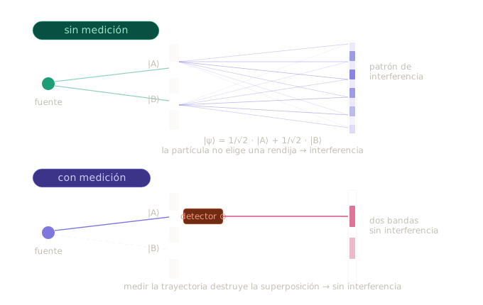
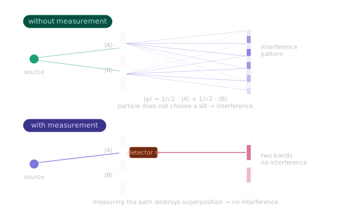
Fire a particle at a barrier with two slits, A and B. Without any measurement of which slit the particle passes through, the particle travels as a linear combination of both paths:

|ψ⟩ = 1/√2 · |A⟩ + 1/√2 · |B⟩

The amplitudes of both paths interfere on the screen. Where they add constructively, you get bright bands. Where they cancel destructively, you get nothing. The characteristic alternating pattern appears.

Now ask which slit the particle went through. The moment you measure the path, the superposition collapses. The particle is in one slit. The interference disappears. Two bands remain, exactly where classical physics would predict them to be.

The particle did not choose a slit and we missed it. The superposition was real, and the measurement ended it.

Tonomura et al. showed in 1989 that this pattern builds up one particle at a time. Each individual particle, traveling in superposition, contributes to the interference. The pattern is not a statistical accident from many particles piling up. It is a property of the quantum state itself.

This is why measurement changes outcomes. Not because the measurement device is poorly calibrated. Because measuring which slit the particle used is precisely what destroys the superposition that was producing the interference.

4. Measurement Destroys Superposition. It Does Not Reveal It.

This is where the coin-under-a-cup analogy breaks, permanently.

The coin analogy suggests the qubit already has a value, and measurement simply reveals it. The uncertainty is yours, not the system's.

Quantum mechanics says something else. The state |ψ⟩ = α|0⟩ + β|1⟩ has no hidden value. It is the complete description of the system. When you measure, the quantum system interacts with the measuring apparatus. The environment entangles with the system. The state collapses irreversibly, probabilistically, to one of the eigenstates.

The result was not predetermined. The act of measuring creates it.

This is not a matter of philosophical preference. The Bell inequalities, proven in 1964 and confirmed experimentally starting in the 1970s, ruled out local hidden variable theories. No pre-existing hidden value can account for the correlations produced by quantum systems. The measurement outcome is genuinely indeterminate before measurement.

What follows:

Each measurement of the same |ψ⟩ can give a different result. This is not imprecision in the equipment. It is fundamental.
Superposition is the real state of the system. There is no hidden fact underneath it waiting to be discovered.
The measurement postulate: after obtaining outcome m, the post-measurement state is the eigenvector of the measured observable associated with m.

The superposition is destroyed by measurement, not decoded.

5. This Is Why Quantum Computing Is Different

Here is where the linear combination stops being abstract.

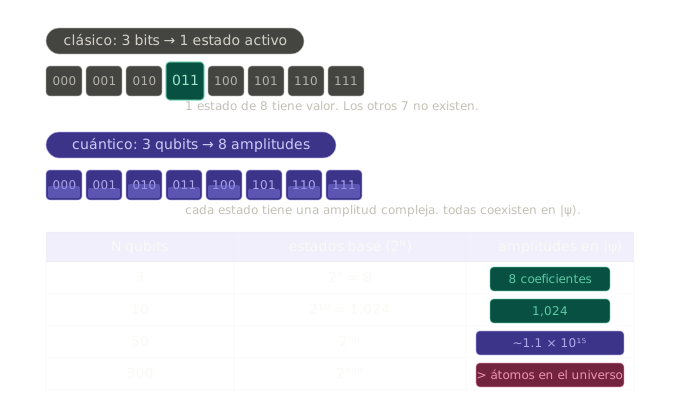
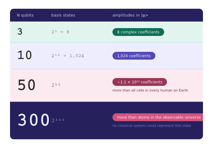
N qubits in superposition represent not one state but 2^N amplitudes simultaneously. A single state vector of N qubits encodes a complex coefficient for every possible N-bit string.

3 qubits: 2³ = 8 basis states → 8 complex amplitudes
10 qubits: 2¹⁰ = 1,024 basis states → 1,024 amplitudes
50 qubits: 2⁵⁰ basis states → ~1.1 × 10¹⁵ amplitudes
300 qubits: 2³⁰⁰ basis states → more than atoms in the observable universe

A classical 3-bit register holds exactly one value. A quantum register of 3 qubits holds a weighted superposition across all 8 possible values, simultaneously, in a single state.

Quantum gates are unitary operations. They act on the entire amplitude vector at once. The algorithm does not run 2^N separate computations in parallel. It manipulates the full amplitude structure through carefully chosen transformations.

The useful analog: a classical die falls on one number. A quantum die exists in superposition of all its outcomes, each carrying an amplitude. The algorithm configures those amplitudes so that the correct result accumulates the highest probability before measurement.

But you cannot read out all 2^N amplitudes. When you measure, you get one outcome, sampled from the probability distribution the algorithm has engineered. The design problem is interference: suppressing wrong answers, amplifying right ones. Grover's algorithm does this for unstructured search. Shor's does it for factorization. Both are interference structures, not classical computations running fast.

This is not a faster classical computer. It is a structurally different computational model operating in a space classical hardware cannot replicate.

What the Framing Gets Wrong, and Why It Matters

"Being 0 and 1 at the same time" is not a harmless simplification. It leads directly to two persistent mistakes.

The first: expecting quantum computers to solve everything faster by trying all options simultaneously. They do not. Speedup is problem-specific and requires algorithm structures that do not exist for most computations.

The second: assuming the engineering challenge is just getting more qubits. It is not. Without coherence, without precise amplitude control, without error correction, more qubits means more noise. The qubit in superposition is fragile, and any unwanted interaction with the environment is effectively a measurement that collapses it.

The next piece in this series is quantum error correction, which is where the real engineering challenge begins. That challenge starts here, with understanding what superposition actually is, and why maintaining it is so hard.

This is part of an ongoing series on quantum computing from the ground up. Previous entries: The End of the Transistor Era · One Story, Two Qubits: Entanglement Explained

Sources

Nielsen, M.A. & Chuang, I.L., Quantum Computation and Quantum Information, Cambridge University Press (2000)
Bloch, F., Nuclear Induction, Physical Review 70 (1946)
Feynman, R., The Feynman Lectures on Physics, Vol. 3, Addison-Wesley (1965)
Tonomura, A. et al., Demonstration of single-electron buildup of an interference pattern, Am. J. Phys. 57 (1989)
Dirac, P.A.M., The Principles of Quantum Mechanics, Oxford University Press (1930)
Preskill, J., Quantum Computing in the NISQ era and beyond (2018)

La superposición no significa que un qubit sea "0 y 1 al mismo tiempo." Es un único objeto matemático — un vector en un espacio de Hilbert complejo — sin valor definido hasta que se mide. Esto es lo que significa realmente, en cinco pasos.

Toda introducción a la computación cuántica comete el mismo error.

"Un qubit puede ser 0 y 1 al mismo tiempo." La frase está en todas partes. Es corta, se mueve rápido, y te da justo la intuición suficiente para sentir que entendiste algo. Pero codifica una imagen fundamentalmente incorrecta de lo que es la superposición, y esa imagen incorrecta se acumula en malentendidos más grandes en cada paso siguiente.

Un qubit en superposición no es "ambos, 0 y 1." Es un único objeto matemático en un estado que no puede reducirse a ninguno de los dos. Esa distinción parece sutil. No lo es.

Esto es lo que está pasando realmente, en cinco pasos.

1. El Estado No Tiene Valor. Tiene un Vector.

Un bit clásico es binario y definitivo. En todo momento, es 0 o 1. Un transistor conduce corriente o no la conduce. El bit siempre tiene un valor.

Un qubit en superposición no tiene valor. Lo que tiene es un estado:

|ψ⟩ = α|0⟩ + β|1⟩

Donde α y β son números complejos llamados amplitudes de probabilidad, sujetos a la condición de normalización:

|α|² + |β|² = 1

Esto no describe dos valores simultáneos. Describe un vector en un espacio de Hilbert complejo de dos dimensiones. El |ψ⟩ es su propia entidad matemática, distinta de |0⟩ y de |1⟩.

Tres cosas se desprenden inmediatamente de esto:

La superposición no significa que el qubit "sea ambos." |ψ⟩ no es una mezcla de |0⟩ y |1⟩ como el gris es mezcla de negro y blanco. Es un tipo de objeto completamente diferente.
α y β son números complejos, no porcentajes. Sus módulos al cuadrado dan probabilidades de medición, pero las amplitudes en sí mismas llevan información de fase que determina la interferencia, y la interferencia es donde vive la computación.
Al medir, el estado colapsa. Obtienes |0⟩ con probabilidad |α|², o |1⟩ con probabilidad |β|². Antes de ese momento, ningún resultado existía.

2. La Esfera de Bloch: Cada Punto Es un Estado Cuántico Posible

Hay una forma geométrica limpia de visualizar todos los estados puros posibles de un qubit. Se llama la esfera de Bloch.

Cualquier estado puro de un qubit puede escribirse usando dos parámetros reales, θ y φ:

|ψ⟩ = cos(θ/2)|0⟩ + e^iφ·sin(θ/2)|1⟩

Estos dos ángulos mapean a un punto único en la superficie de una esfera unitaria:

Polo norte (θ = 0): el estado |0⟩. Medir da 0 con 100% de certeza.
Polo sur (θ = π): el estado |1⟩. 100% de probabilidad de medir 1.
Ecuador (θ = π/2): superposición máxima, 50% de probabilidad para cada resultado.

Pero la esfera de Bloch muestra algo que los números de probabilidad solos no muestran. El ángulo φ es la fase relativa. No cambia las probabilidades de medición en absoluto. Dos estados en el ecuador con φ = 0 y φ = π dan resultados 50/50 en cada medición. Sin embargo, son estados diferentes, y se comportan de manera completamente diferente dentro de un algoritmo, porque la fase determina la interferencia.

Un estado que parece idéntico desde afuera puede producir resultados computacionales completamente diferentes. Esto no es un quirk. Es el mecanismo.

3. La Doble Rendija: Donde la Superposición Se Vuelve Visible

La demostración física más clara de la superposición y la interferencia es el experimento de la doble rendija.

Dispara una partícula hacia una barrera con dos rendijas, A y B. Sin ninguna medición de por cuál rendija pasa la partícula, esta viaja como combinación lineal de ambas trayectorias:

|ψ⟩ = 1/√2 · |A⟩ + 1/√2 · |B⟩

Las amplitudes de ambas trayectorias interfieren en la pantalla. Donde se suman constructivamente, aparecen bandas brillantes. Donde se cancelan destructivamente, no hay nada. El característico patrón alternado aparece.

Ahora pregunta por cuál rendija pasó la partícula. En el momento en que mides la trayectoria, la superposición colapsa. La partícula está en una sola rendija. La interferencia desaparece. Quedan dos bandas, exactamente donde la física clásica las predice.

La partícula no eligió una rendija mientras no mirábamos. La superposición era real, y la medición la terminó.

Tonomura et al. demostraron en 1989 que este patrón se construye una partícula a la vez. Cada partícula individual, viajando en superposición, contribuye a la interferencia. El patrón no es un accidente estadístico de muchas partículas acumulándose. Es una propiedad del estado cuántico en sí.

Por eso la medición cambia los resultados. No porque el aparato de medición esté mal calibrado. Porque medir por cuál rendija pasó la partícula es precisamente lo que destruye la superposición que estaba produciendo la interferencia.

4. La Medición Destruye la Superposición. No la Revela.

Aquí es donde la analogía de la moneda bajo una taza se rompe permanentemente.

La analogía de la moneda sugiere que el qubit ya tiene un valor, y la medición simplemente lo revela. La incertidumbre es tuya, no del sistema.

La mecánica cuántica dice otra cosa. El estado |ψ⟩ = α|0⟩ + β|1⟩ no tiene un valor oculto. Es la descripción completa del sistema. Al medir, el sistema cuántico interactúa con el aparato de medición. El entorno se entrelaza con el sistema. El estado colapsa irreversiblemente, probabilísticamente, a uno de los autoestados.

El resultado no estaba predeterminado. El acto de medir lo crea.

Esto no es una cuestión de preferencia filosófica. Las desigualdades de Bell, demostradas en 1964 y confirmadas experimentalmente desde los años 70, descartaron las teorías de variables ocultas locales. Ningún valor oculto preexistente puede dar cuenta de las correlaciones producidas por los sistemas cuánticos. El resultado de la medición es genuinamente indeterminado antes de medir.

Lo que se desprende:

Cada medición del mismo |ψ⟩ puede dar un resultado diferente. Esto no es imprecisión del equipo. Es fundamental.
La superposición es el estado real del sistema. No hay un hecho oculto debajo de ella esperando ser descubierto.
El postulado de la medición: tras obtener el resultado m, el estado post-medición es el autovector del observable medido asociado a m.

La superposición es destruida por la medición, no decodificada.

5. Por Eso la Computación Cuántica Es Diferente

Aquí es donde la combinación lineal deja de ser abstracta.

N qubits en superposición representan no un estado sino 2^N amplitudes simultáneamente. Un único vector de estado de N qubits codifica un coeficiente complejo para cada cadena de N bits posible.

3 qubits: 2³ = 8 estados base → 8 coeficientes complejos
10 qubits: 2¹⁰ = 1,024 estados base → 1,024 coeficientes
50 qubits: 2⁵⁰ estados base → ~1.1 × 10¹⁵ coeficientes
300 qubits: 2³⁰⁰ estados base → más átomos que en el universo observable

Un registro clásico de 3 bits sostiene exactamente un valor. Un registro cuántico de 3 qubits sostiene una superposición ponderada sobre los 8 valores posibles, simultáneamente, en un solo estado.

Las compuertas cuánticas son operaciones unitarias. Actúan sobre el vector de amplitud completo de una sola vez. El algoritmo no ejecuta 2^N cómputos separados en paralelo. Manipula la estructura completa de amplitudes a través de transformaciones cuidadosamente elegidas.

La analogía útil: un dado clásico cae en un número. Un dado cuántico existe en superposición de todos sus resultados, cada uno con una amplitud. El algoritmo configura esas amplitudes para que el resultado correcto acumule la mayor probabilidad antes de medir.

Pero no puedes leer las 2^N amplitudes. Al medir, obtienes un resultado, muestreado de la distribución de probabilidad que el algoritmo construyó. El problema de diseño es la interferencia: suprimir las respuestas incorrectas, amplificar las correctas. El algoritmo de Grover hace esto para búsqueda no estructurada. El de Shor para factorización. Ambos son estructuras de interferencia, no cómputos clásicos ejecutándose rápido.

Esto no es una computadora clásica más rápida. Es un modelo computacional estructuralmente diferente, que opera en un espacio que el hardware clásico no puede replicar.

Lo Que el Encuadre Habitual Distorsiona, y Por Qué Importa

"Ser 0 y 1 al mismo tiempo" no es una simplificación inofensiva. Lleva directamente a dos errores persistentes.

El primero: esperar que las computadoras cuánticas resuelvan todo más rápido probando todas las opciones simultáneamente. No es así. La ventaja cuántica es específica al problema y requiere estructuras de algoritmos que no existen para la mayoría de las computaciones.

El segundo: asumir que el desafío de ingeniería es simplemente conseguir más qubits. No lo es. Sin coherencia, sin control preciso de amplitudes, sin corrección de errores, más qubits significa más ruido. El qubit en superposición es frágil, y cualquier interacción no deseada con el entorno es efectivamente una medición que lo colapsa.

La siguiente pieza de esta serie es la corrección de errores cuánticos, que es donde comienza el verdadero desafío de ingeniería. Ese desafío empieza aquí, entendiendo qué es realmente la superposición, y por qué mantenerla es tan difícil.

Esta es parte de una serie continua sobre computación cuántica desde cero. Entradas anteriores: El Fin de la Era del Transistor · Una Historia, Dos Qubits: El Entrelazamiento Explicado

Fuentes

Nielsen, M.A. & Chuang, I.L., Quantum Computation and Quantum Information, Cambridge University Press (2000)
Bloch, F., Nuclear Induction, Physical Review 70 (1946)
Feynman, R., The Feynman Lectures on Physics, Vol. 3, Addison-Wesley (1965)
Tonomura, A. et al., Demonstration of single-electron buildup of an interference pattern, Am. J. Phys. 57 (1989)
Dirac, P.A.M., The Principles of Quantum Mechanics, Oxford University Press (1930)
Preskill, J., Quantum Computing in the NISQ era and beyond (2018)

A Qubit Is Not 0 or 1. It Is a Linear Combination of Both. Un Qubit No Es 0 ni 1. Es una Combinación Lineal de Ambos.